
Snowflake continues to set the standard for Data in the Cloud by taking away the need to perform maintenance tasks on your data platform and giving you the freedom to choose your data model methodology for the cloud. Snowflake is a massively parallel platform (MPP) through its proprietary technologies. In this blog post we will explain how to make use of a technique unique to Snowflake to efficiently query large satellite tables for the current record by a parent key (hub or link).
This post is number 4 in our “Data Vault Techniques on Snowflake” series:
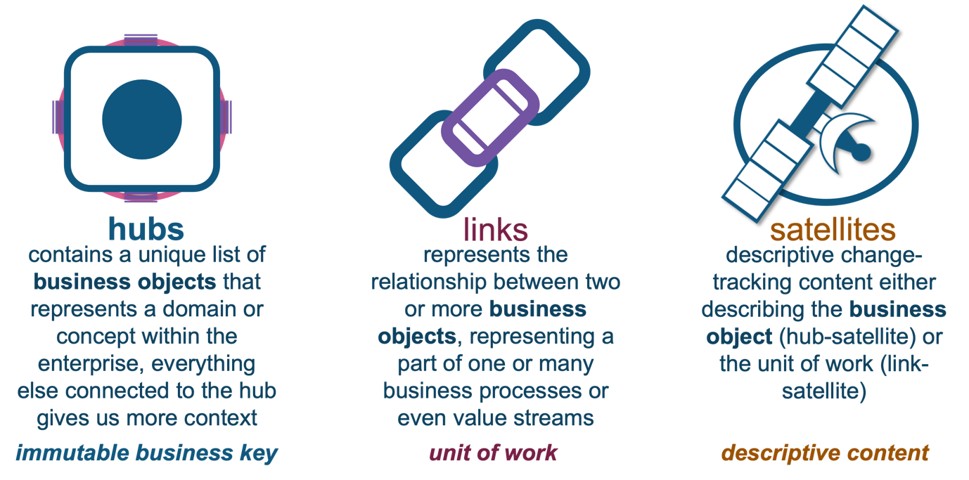
First, a quick reminder of the different data vault table types:
We will use a variation of one of the query-assistance tables available to us for improving query performance, the PIT table.

In the first post of this series, we explored how Data Vault 2.0 and its INSERT-ONLY modeling technique is very well suited to how Snowflake stores its table in the form of micro-partitions. Data Vault satellite tables provide the change history for its parent entity (hub or link); this is important for historical analysis and audit history, but most analytics from a data platform will be concerned with the current state of the parent entity.
As we saw in that first post, Data Vault 2.0 satellite tables do not have an end-date column; therefore, to fetch the current state of the parent entity we must use the LEAD window function to QUALIFY which is the current record on all the underlying micro-partitions.
Why?Let’s relook at this diagram from the first post:

As we see the satellite table grow, it captures newer state data of the parent entity. For a given entity, its current state could be in a much older micro-partition than the rest. Essentially, the profile of current records in this satellite table is scattered, and Snowflake would indeed have to scan every micro-partition to determine the current state record for a given entity.
For the remainder of this post, the satellite table being queried contains 61 million records, but only 1.9 million records in this satellite represent the current state of a hub parent key. Also, we flush the virtual warehouse between test runs and have disabled Snowflake Result Cache to keep the query runtime results consistent for a fair comparison.

Snowflake maintains a hot pool of XSMALL virtual warehouses ready for a user-role to spin up and start using, which is why query runs are initiated near instantaneously for an XSMALL-sized virtual warehouse. Noted in the above query profile, the query needed to scan all micro-partitions of the satellite table to return 1.9M records; the query ran for 50 seconds. Not bad for a newly spun up virtual warehouse that falls within the 60 seconds minimum credit charge for a virtual warehouse!
Have we wasted 10 seconds, or could those 10 seconds have been used for other queued queries? Can we improve on this performance?
Let’s try by upsizing the virtual warehouse to X4LARGE T-shirt size.

Notice that the first run executed for well over 2 minutes. What happened? Snowflake does not maintain a hot pool of X4LARGE virtual warehouses for on-demand accounts. Instead, these need to be spun up. However, upon the second run (and we flushed the cache once again) the query did run for 5.5 seconds, a 100% improvement on the second run! But we still must scan all micro-partitions of the very big satellite table but using far more nodes.
Each upsize of a virtual warehouse doubles the number of nodes in a cluster and thus doubles the credit expenditure. For example:
| Virtual Warehouse T-Shirt Size | Number of Nodes = Credits Charged Per Hour | Credits Charged Per Second |
|---|---|---|
| XSMALL | 1 | 0.0003 |
| SMALL | 2 | 0.0006 |
| … | … | … |
| X4LARGE | 128 | 0.0356 |
Click here to see full warehouse size chart.
Note: X4LARGE (and all other T-shirt sizes) would only bill for running time, not the time it takes for the virtual warehouse to spin up.
What could we do differently?
Storage in the cloud is cheap, and by using Snowflake’s encrypted, compressed proprietary columnar and row-optimized tables, it is even cheaper. In 2021 Snowflake announced improvements to its data storage compression algorithms that reduced Snowflake’s table storage footprint even further. The cost of storage on disk is a cost Snowflake incurs that is passed on to its customers. This means Snowflake achieves a smaller storage footprint than an equivalent table in another blob store and does not charge you for those savings, but instead passes those savings on to you
Let’s look at data model and object options:
1. Materialized View is a pre-computed data set derived from a query specification and stored for later use. Essentially, underneath a materialized view (MV) is the persistence of micro-partitions clustered in a way to better suit the type of queries that will be executed on that data itself. We’d love to have the current records clustered together so that the query plan references the least number of micro-partitions to answer that query. The problem with a current limitation of MVs is that it does not allow for window functions such as LEAD(), and therefore it’s not possible to infer the current record for a satellite table. Snowflake MVs also do not allow for join conditions and therefore cannot be used with a PIT table.
2. Search Optimization Service (SOS) aims to significantly improve the performance of selective point lookup queries on tables. A point lookup query returns only one or a small number of distinct rows. SOS is like a secondary index when clustering is not a feasible option, but for a small number of records this does not fall into the scope of retrieving millions of current records from a satellite table. In fact, after testing and allowing SOS to build its search access paths, attempting a query to find the current record for a parent entity does not use SOS at all. It is absent from the query profile and therefore SOS is not effective for this type of query.
3. Streams is a change data capture mechanism that places a point-in-time reference (called an offset) as the current transactional version of the object. Although an excellent way of tracking new records in a table, streams have no concept of the table content itself. Once a stream is consumed, the offset moves to the end of the table indicating that all the records since it was last processed are now consumed. (We do have a use for streams in Data Vault as seen in blog post #2, and as we will also see in post #5.)

4. Un-deprecating end dates for Data Vault 2.0 (the constant gardener suggestion) – A satellite table’s attributes can be a single column to as many as hundreds of columns. In post #1 we explained why we prefer not to persist end dates, and even adding the end date and clustering by that end date implies backend processing to keep the satellite clustered in end-date order. The preferred Data Vault 2.0 pattern leaves data in the order it arrives (load order) and does not need to run a serverless process to keep the order up to date. However, this suggestion does have merit. What is the outcome of adding that end date? More table churn and a serverless cost to maintain that clustering key order, but the satellite table order is maintained as a service (credit consumption) and you will query the fewest micro-partitions and even use fewer micro-partitionsbecause Snowflake is constantly “trimming the hedges.” The downside, of course, is if the satellite table starts to grow into the billions of records, what will be the cost to keep trimming these hedges?
Notice how few micro-partitions there are. But the fact that there are fewer micro-partitions that make up a table is because they are constantly being maintained whenever there is an update. For a high-churn table with Time -Travel and Fail-Safe enabled, the costs could escalate and you want this data protection for your auditable tables. A query on this satellite table will use what is called static pruning by specifying the filter condition (WHERE end-date = high-date) to get to the current record-per-parent entity.
Part 2 of 2 on query optimization: understanding JoinJilter
For the eagle-eyed reader, in the previous blog post we indeed did see something in the query plan that deserves an explanation: JoinFilter[6]:

It’s a little underwhelming because in that case the use of a JoinFilter did not filter anything at all. Why? Because we were using a daily PIT table. The daily PIT table in our example contained all the keys and load dates needed to pull in all the data from surrounding satellite tables, and for this example, this was not very useful.
However, as noted earlier, most queries out of a data analytics platform in fact deal with the current record for a business object or unit of work. JoinFilter is used to achieve something called dynamic pruning, and that is to establish a point-in-time lookup table that informs Snowflake’s query planner where to locate the current record for a parent key. We will call this the current point-in-time table, or C-PIT.

We achieve the same outcome as the satellite table with the end-date by applying a join between a C-PIT and the satellite table itself. Yes, you are in essence maintaining an additional table, but it can be loaded in parallel and the satellite table itself does not need to be constantly maintained after every satellite table update. In addition, you are not churning more micro-partitions than you need with UPDATE statements because the satellite table remains INSERT-ONLY and therefore enjoys the protections of Time Travel and Fail-Safe without the potential for high churn. C-PIT can also be updated only when it is needed—think about it.
Let’s illustrate the deployment of C-PIT:

The design behind a C-PIT will be:
- Populated in parallel from the same source using the same mechanism to detect changes idempotently, the record-hash (aka HashDiff).
- A C-PIT exists for each satellite table needing an efficient querying mechanism, typically high-churn and large satellite tables.
- C-PIT will contain the business key if it is supporting a hub-satellite table, or the relationship keys if it is supporting a link-satellite table.
- C-PIT will contain the satellite’s hash key, load date, and record hash and nothing else; the satellite table has the same Data Vault metadata tags but also (of course) the attributes of the parent entity. These could range from one attribute to hundreds.
- Unlike the satellite table, a C-PIT is disposable and therefore does not need the same protection as its related satellite table. Therefore, the table is defined as transient and does not have Fail-Safe or Time Travel beyond 1 day. It can deal with data loaded at any cadence because high churn is not a concern. The satellite table remains INSERT-ONLY.
- C-PIT is used in an equi-join to locate the current record from its accompanying satellite table.
- C-PIT is updated using a MERGE statement and keeps no history, it is only concerned with the current record and therefore keeps the active/current load date per parent key and that entity’s HashDiff. Remember a satellite’s HashDiff is defined in staging as illustrated above—it can be sent to two destinations, the satellite table, and the C-PIT table respectively.
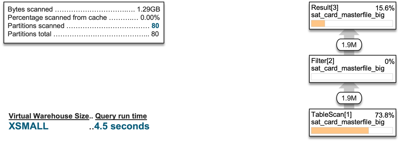
Could we improve on 4.5 seconds by upsizing the virtual warehouse?

No! Using a larger virtual warehouse with the JoinFilter was slower than using an XSMALL virtual warehouse. Why? Snowflake needs to allocate work to each node in the virtual warehouse cluster; the larger the virtual warehouse T-shirt size, the more nodes Snowflake needs to orchestrate and schedule work to. That of course adds latency to the query response time.
Lab report
This blog post is not intended to apply to your own experiments and doesn’t assume the solutions presented above will resolve all situations. The intention here is to give you various options to consider as you look to understand the possibilities of performance of the Data Cloud. It is important that you establish a repeatable pattern that has as few “switches” as possible, and by switches I mean don’t design an architecture that follows a different automation path depending on minor factors that adds unnecessary complexity to your data flow. This will inevitably lead to technical debt.
In the next blog post we will look at an architecture approach that exclusively uses Snowflake proprietary technology to achieve near real-time data pipelines.